MATLAB¶

Overview¶

The gmm_occupancy_modeling_examples package contains MATLAB scripts for sampling from GMMs and updating an occupancy grid map for an entire dataset of a mine.

Initialize the MATLAB Environment¶

When starting up MATLAB, make sure to run the workon.m script in the top level directory. This will add all required MATLAB packages to your path.

matlab> cd gira3d-occupancy-modeling
matlab> workon

Download Data¶

The data directory contains a script that you will need to execute in order to download all of the data associated with this tutorial.

pip install gdown
cd gira3d-occupancy-modeling/data
./download.sh

The complete dataset is < 200MB so it should download fairly quickly.

Running the Example¶

After running the workon script, execute the following MATLAB to run the example

matlab> cd wet/src/gmm_occupancy_modeling_example/matlab/
matlab> occupancy_modeling_example

This example uses the default grid cell size of 0.2m. To update the grid extents, you will need to run the determine_grid_parameters.m script for the paramters that you want and then update them in the yaml file. Unfortunately, MATLAB doesn't have built-in yaml handling, so for now the process is not fully automated.

Detailed Explanation of the Script¶

First, we initialize the Grid3D data structure. Note the grid3d software does not currently support dynamic grid resizing so please ensure the start and end points of your point cloud all lie within the grid extents.

grid = Grid3D(PATH_TO_CONFIG);

PATH_TO_CONFIG specifies the location of the yaml file, which contains the grid3d parameters.

gmm = GMM3();
gmm.load([GMM_DIR, num2str(i), '.gmm']);
pcld = gmm.sample(1e5);

The lines above load the GMM file and sample 10,000 points.

tpcld = transpose(R*transpose(pcld) + repmat(t, 1, size(pcld,1)));

The points are transformed into world coordinates using the ground truth data stored in odometry.mat.

for j = 1:size(tpcld,1)
  st = t;
  en = transpose(tpcld(j,:));
  trimmed_max_range = max_range - resolution;
  grid.addRay(st, en, trimmed_max_range);
end

Add each point to the grid map.

% Plot the output
[xyz, probabilities] = grid.getXYZProbability();

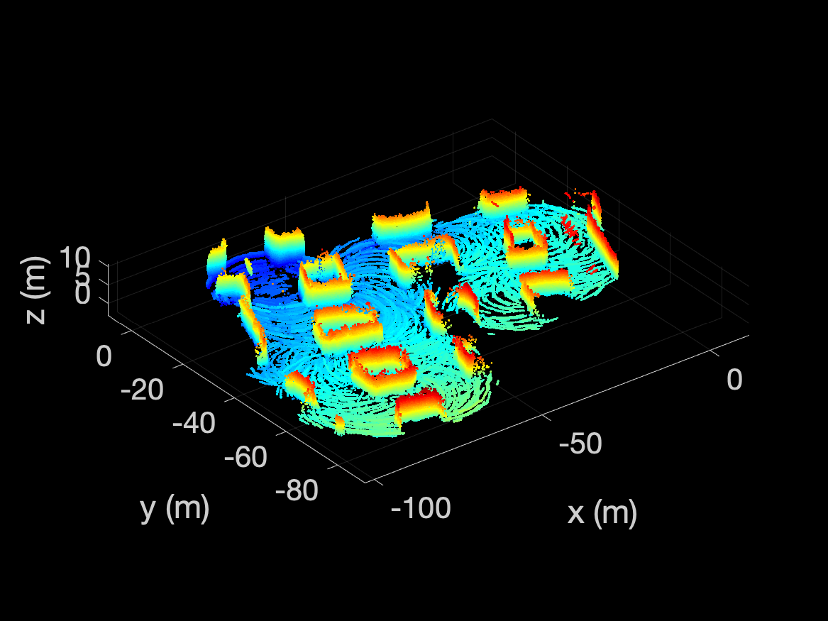
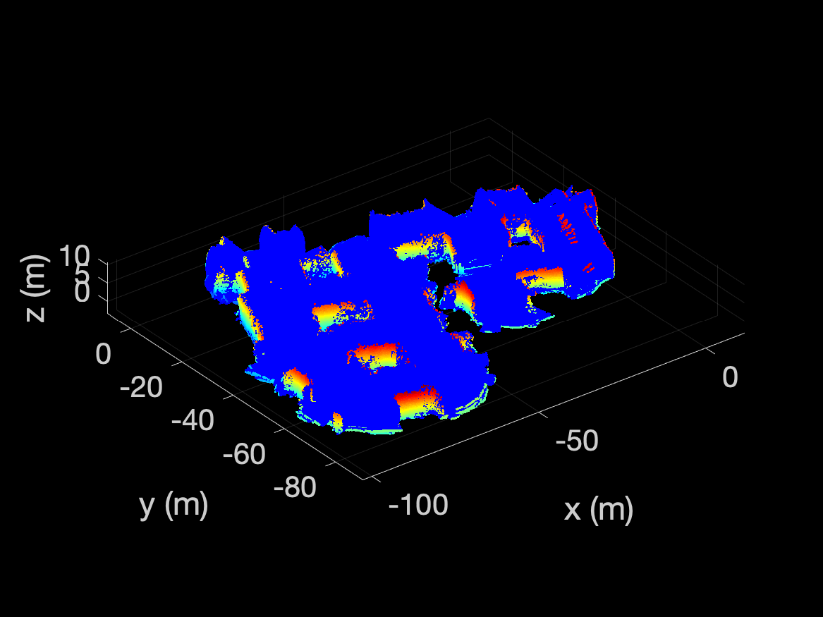
if (PLOT_OCCUPIED_POINTS)
  occupied_indices = find(probabilities >= OCCUPIED_THRESH);
  occupied_pts = transpose(xyz(:, occupied_indices));
  pcshow(occupied_pts);
  colormap('jet');
end

if (PLOT_FREE_POINTS)
  free_indices = find(probabilities <= FREE_THRESH);
  free_pts = transpose(xyz(:, free_indices));
  pcshow(pointCloud(free_pts, 'Color', repmat([0, 0, 1], size(free_pts,1), 1)));
end

The occupied and free points are plotted using these lines and should look like the following: Plotting occupied points Plotting free space points

Visualization¶

Scripts are provided to visualize GMMs. A GMM may be visualized by loading from file and using the plot function in the GMM3.m file. An example is provided below:

matlab> gmm = GMM3();
matlab> gmm.load('/path/to/data/mine_001_part3/100_components/400.gmm');
matlab> gmm.plot([0,0,1]) # Provide color for the GMM using [R, G, B] values between 0 and 1
matlab> pcld = load('/path/to/data/mine_001_part3/pointclouds/400.txt');
matlab> hold on; pcshow(pcld); colormap(flipud(jet));

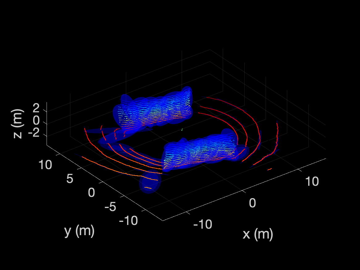
Plotting the GMM on top of a pointcloud

The number of sigmas on the covariance can be adjusted by opening the GMM3.m script and changing nsigmas. The alpha can be changed by updating the alpha. The color is supplied in the plot() function call.

Operating Systems¶

These tutorials have been tested on the following operating systems:

Ubuntu 20.04
Ubuntu 18.04