MATLAB

Overview

The following packages are used for the MATLAB tutorial: gmm_d2d_registration_matlab, gmm_d2d_registration_examples, and gmm.

The gmm_d2d_registration_examples package contains MATLAB scripts for registering a single pair of GMMs. It also contains scripts for processing entire datasets.

Initialize the MATLAB Environment

The tutorial uses mtimesx, which is compiled and build in the set of dry packages. A shared library is created and installed in the dry/install directory. In order to load this library properly, you will need to run the workon script to find it and add its containing directory to the MATLAB path. To do this use the included workon.m file. This file also adds the matlab directories containing MATLAB scripts and functions to the path.

matlab> cd gira3d-registration
matlab> workon

Download Data

The data directory contains a script that you will need to execute in order to download all of the data associated with this tutorial.

shell> pip install gdown 
shell> cd gira3d-registration/data
shell> ./download.sh

The complete dataset is quite large so be prepared for this to take some time.

Registering a Pair of GMMs

The data directory contains a subdirectory called pair that contains two example GMMs: source.gmm and target.gmm. In order to run the GMM registration code, do the following in matlab.

matlab> cd wet/src/gmm_d2d_registration_examples/matlab
matlab> registration_example

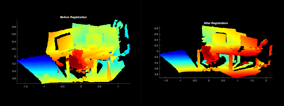
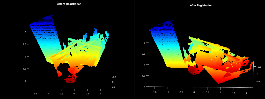
Two MATLAB figures will also display with the registration output using the original pointclouds (note: not the GMMs).

Detailed Explanation of the Script

First, an isoplanar registration is run to overcome local minima:

x_opt = zeros(6,1);
[x_opt, score] = isoplanar_registration(source_file, target_file, zeros(6,1));

x_opt is the registration result consisting. A refinement step is run using the following function call:

[x_opt, score] = anisotropic_registration(source_file, target_file, x_opt);

The 3x3 rotation matrix and translation vector are extracted using:

Rotation = axang2rotm([x_opt(4:6) / norm(x_opt(4:6)); norm(x_opt(4:6))]');
translation = x_opt(1:3);

An explanation of the visualization is found in in the visualization section.

TUM Registration

To run the full TUM registration pipeline with pre-made GMMs, you can use the script in gmm_d2d_registration_examples/matlab/run_tum_dataset.m.

matlab> run_tum_dataset

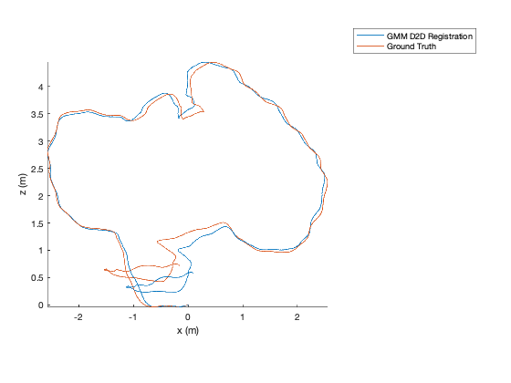
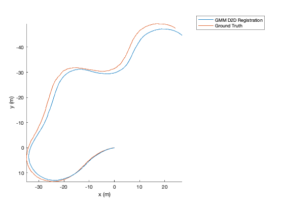
The result will be the trajectory generated from frame-to-frame registration with the ground truth plotted on top.

Cave Registration

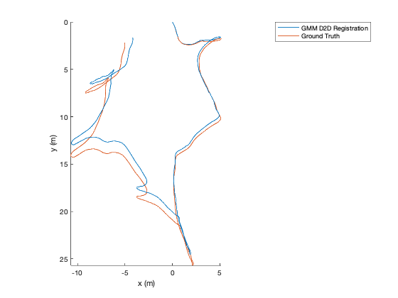
To run the cave dataset with pre-made GMMs, you can use the script in gmm_d2d_registration_examples/matlab/run_cave_dataset.m.

matlab> run_cave_dataset

Mine Registration

To run the cave dataset with pre-made GMMs, you can use the script in gmm_d2d_registration_examples/matlab/run_mine_dataset.m.

matlab> run_mine_dataset

Closing the loop and using Pose Graphs

Software is provided with an example of how to close the loop.

pose_graph_example

The result will be a video that looks like the following:

where ground truth is in white and the pose graph trajectory is shown in red or purple. Purple means a loop closure constraint was added.

Visualization

Scripts are provided to visualize GMMs. A GMM may be visualized by loading from file and using the plot function in the GMM3.m file. An example is provided below:

matlab> gmm = GMM3();
matlab> gmm.load('/path/to/data/rgbd_dataset_freiburg3_long_office_household/100_components/1200.gmm');
matlab> gmm.plot([1,0,0]) # Provide color for the GMM using [R, G, B] values between 0 and 1
matlab> pcld = load('/path/to/data/rgbd_dataset_freiburg3_long_office_household/pointclouds/1200.txt');
matlab> hold on; pcshow(pcld); colormap(flipud(jet));

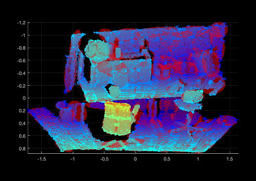
The number of sigmas on the covariance can be adjusted by opening the GMM3.m script and changing nsigmas. The alpha can be changed by updating the alpha. The color is supplied in the plot() function call.

Operating Systems

These tutorials have been tested on the following operating systems:

• Ubuntu 20.04
• Ubuntu 18.04