Point Cloud Modeling using Self-Organizing Gaussian Mixture Models (SOGMM)
This tutorial presents modeling a point cloud using the SOGMM approach presented in [1]. We assume that a depth-intensity point cloud with $N$ points (i.e., point cloud is a set of $N$ four-dimensional points $\mathbf{x}$) is given. The output is a Gaussian Mixture Model (GMM) of the point cloud that can be used for:
- Inference for intensity image reconstruction
- Dense sampling for 3D point cloud reconstruction
Input
For the purposes of this tutorial, download the point cloud data from
this link. The
downloaded zip folder contains point cloud data from a few frames of the
stonewall, copyroom, and lounge ICL-NUIM datasets [2].
Extract the zip folder. You will get a folder with files named like this:
gira3d-tutorial-data
├── pcd_copyroom_2364_decimate_1_0.pcd
├── pcd_copyroom_2364_decimate_2_0.pcd
└── ...
The files are named as pcd_<dataset-name>_<frame-number>_decimate_<decimation_amount>.pcd.
Here, decimation of 1.0 means the original image of size 640 x 480 was used to generate the point cloud.
Likewise, decimations of 2.0, 3.0, and 4.0 correspond to image sizes 320 x 240, 213 x 160, and
160 x 120 respectively.
For the purposes of this tutorial, we limit to the frames provided in the folder above. However, the methodology will work on any registered depth-intensity image pair.
Learning the SOGMM Model
We start by importing the run time dependencies:
%matplotlib inline
import numpy as np
import open3d as o3d

from sogmm_py.utils import read_log_trajectory, o3d_to_np, np_to_o3d
from sogmm_py.vis_open3d import VisOpen3D
For the purposes of this tutorial, we will use frame 1763 of the lounge dataset.
frame = 1763
datasetname = 'lounge'
Import a ground truth point cloud from the dataset folder.
pcld_gt = o3d.io.read_point_cloud('./gira3d-tutorial-data/pcd_' +
                                  str(datasetname) +
                                  '_' + str(frame) +
                                  '_decimate_1_0.pcd', format='pcd')
pcld_gt_np = o3d_to_np(pcld_gt)
Import the ground truth SE(3) pose.
traj = read_log_trajectory('./gira3d-tutorial-data/' +
                           str(datasetname) + '-traj.log')
pcld_pose = traj[frame].pose
Initialize the intrinsics matrix and width and height variables.
K = np.eye(3)
K[0, 0] = 525.0
K[1, 1] = 525.0
K[0, 2] = 319.5
K[1, 2] = 239.5

W = (int)(640)
H = (int)(480)
To visualize, please use our python wrapper over the Open3D visualizer.
vis = VisOpen3D(visible=True)
vis.visualize_pcld(pcld_gt, pcld_pose, K, W, H)
vis.render()
del vis
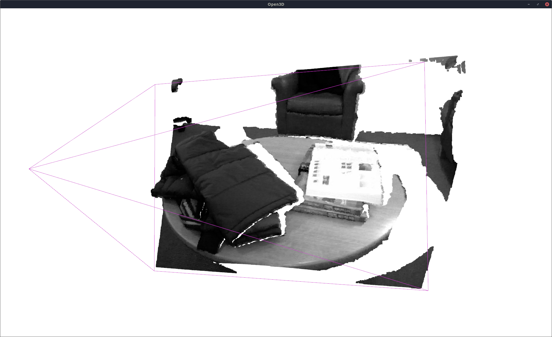
You should see an interactive Open3D window that shows the depth-intensity point cloud and the camera frustrum:

Since the SOGMM method produces a generative model of the point cloud, we can train it on decimated point clouds. In this example, let us use a decimation of 4.0.
deci = 4.0
Get the decimated point cloud from the dataset folder:
pcld_deci = o3d.io.read_point_cloud('./gira3d-tutorial-data/pcd_' +
                                  str(datasetname) +
                                  '_' + str(frame) +
                                  '_decimate_' +
                                  str(deci).replace('.', '_') +
                                  '.pcd', format='pcd')
pcld_deci_np = o3d_to_np(pcld_deci)
Initialize the intrinsics matrix and width and height variables corresponding to the decimation factor.
K_d = np.eye(3)
K_d[0, 0] = 525.0/deci
K_d[1, 1] = 525.0/deci
K_d[0, 2] = 319.5/deci
K_d[1, 2] = 239.5/deci

W_d = (int)(640/deci)
H_d = (int)(480/deci)
Visualize the decimated point cloud the same way.
vis = VisOpen3D(visible=True)
vis.visualize_pcld(pcld_deci, pcld_pose, K_d, W_d, H_d)
vis.render()
del vis
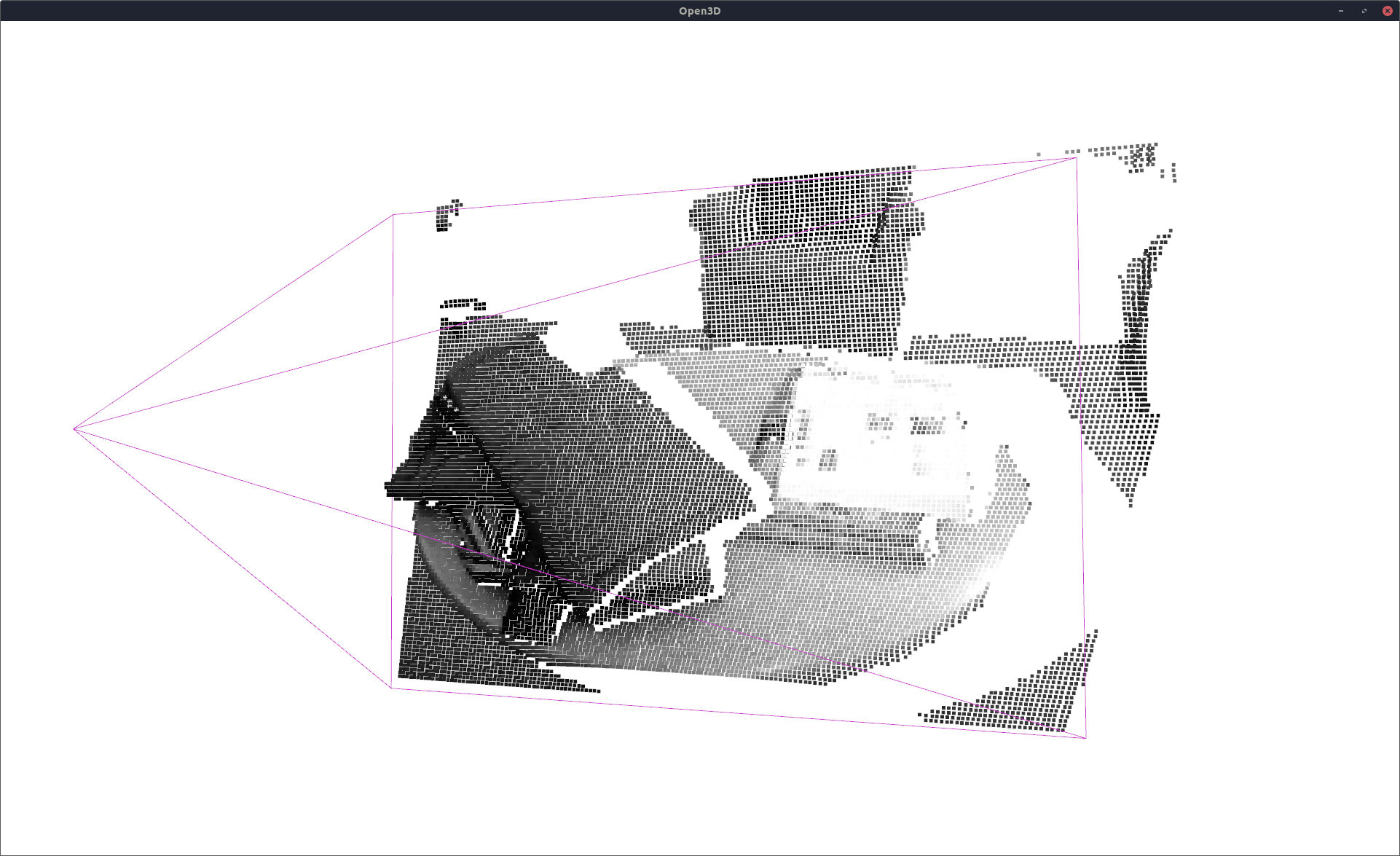
The decimated point cloud looks like this:

Next, we learn a SOGMM on the decimated point cloud. Both CPU-only and GPU-accelerated cases are supported. Both of these modules can be accessed through the SOGMM class.
from sogmm_py.sogmm import SOGMM
SOGMM CPU
%%time
sg_cpu = SOGMM(bandwidth=0.02, compute='CPU')
model_cpu = sg_cpu.fit(pcld_deci_np)
Compute platform is CPU
CPU times: user 2min 6s, sys: 8.13 s, total: 2min 14s
Wall time: 22.5 s
We can take a look at the number of components automatically chosen by SOGMM for this frame:
model_cpu.n_components_
639
SOGMM GPU
%%time
sg_gpu = SOGMM(bandwidth=0.02, compute='GPU')
model_gpu = sg_gpu.fit(pcld_deci_np)
Compute platform is GPU
CPU times: user 3.87 s, sys: 5.88 s, total: 9.75 s
Wall time: 2.91 s
Let us make sure we got the same number of components.
model_gpu.n_components_
639
Inference for Intensity Image
Intensity image can be constructed using the conditional GMM as follows. For more details on how the conditional distribution is computed, please refer to [1].
%%time
_, expected_intensities, _ = model_gpu.color_conditional(pcld_gt_np[:, 0:3])
CPU times: user 1min 33s, sys: 468 ms, total: 1min 34s
Wall time: 5.66 s
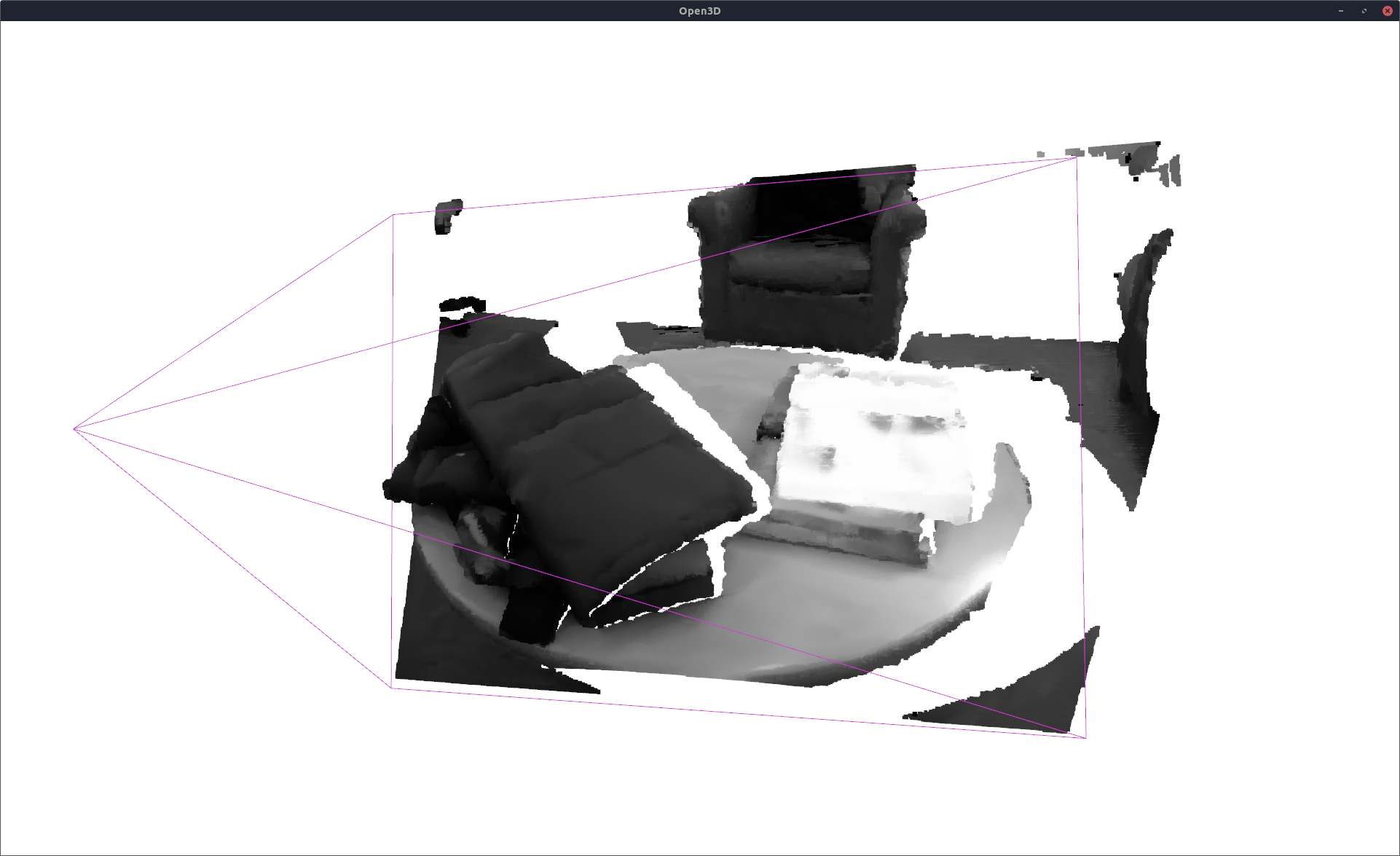
expected_intensities contains the expected intensity values at the ground truth 3D points. Let us visualize these reconstructed intensity values.
recon_pcld = np.zeros(pcld_gt_np.shape)
recon_pcld[:, 0:3] = pcld_gt_np[:, 0:3] # we are constructing intensity image on gt 3D points
recon_pcld[:, 3] = np.squeeze(expected_intensities)

vis = VisOpen3D(visible=True)
vis.visualize_pcld(np_to_o3d(recon_pcld), pcld_pose, K, W, H)
vis.render()
del vis

Higher accuracy can be achieved if the learning is performed at a lower deci value (at the cost of higher computation time).
Dense sampling for 3D point cloud reconstruction
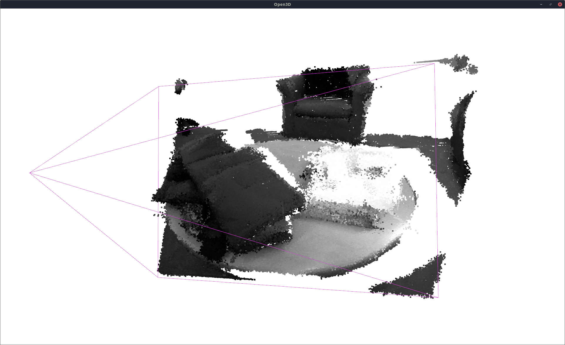
Dense sampling from the 4D GMM can be performed using the usual Box-Mueller sampling method [3].
resampled_pcld = sg_gpu.joint_dist_sample(pcld_gt_np.shape[0]) # sample 4D points from the model
vis = VisOpen3D(visible=True)
vis.visualize_pcld(np_to_o3d(resampled_pcld), pcld_pose, K, W, H)
vis.render()
del vis

Performance Measures
We support computing the following:
- Peak Signal-To-Noise Ratio (PSNR): To measure the accuracy of intensity image reconstruction.
- Structure Similarity Index Measure (SSIM): To measure the accuracy of intensity image reconstruction.
- F-score: To measure the accuracy of resampled point cloud.
- Precision: To measure the accuracy of resampled point cloud.
- Recall: To measure the accuracy of resampled point cloud.
- Mean Reconstruction Error (MRE): To measure the accuracy of resampled point cloud.
- Std. Dev. Reconstruction Error: To measure the accuracy of resampled point cloud.
- Memory: To measure the compactness.
from sogmm_py.utils import calculate_depth_metrics, calculate_color_metrics
fsc, pre, re, rm, rs = calculate_depth_metrics(pcld_gt, np_to_o3d(resampled_pcld))
print("fscore %f precision %f recall %f recon. mean %f recon. std. dev. %f" % (fsc, pre, re, rm, rs))

from sogmm_py.utils import ImageUtils
iu = ImageUtils(K) # image manipulation utility
_, gt_g = iu.pcld_wf_to_imgs(pcld_pose, pcld_gt_np) # project gt pcld on camera
if np.isnan(gt_g).any():
    gt_g = np.nan_to_num(gt_g)
_, pr_g = iu.pcld_wf_to_imgs(pcld_pose, recon_pcld) # project recon pcld on camera
if np.isnan(pr_g).any():
    pr_g = np.nan_to_num(pr_g)
psnr, ssim = calculate_color_metrics(gt_g, pr_g) # compare the intensity images
print("psnr %f ssim %f" % (psnr, ssim))
fscore 0.963304 precision 0.977305 recall 0.949698 recon. mean 0.002654 recon. std. dev. 0.002685
psnr 28.332349 ssim 0.869796
# computing memory usage
M = model_gpu.n_components_
mem_bytes = 4 * M * (1 + 10 + 4)
print('memory %d bytes' % (mem_bytes))
memory 38340 bytes
References
[1] K. Goel, N. Michael, and W. Tabib, “Probabilistic Point Cloud Modeling via Self-Organizing Gaussian Mixture Models,” IEEE Robotics and Automation Letters, vol. 8, no. 5, pp. 2526–2533, May 2023, doi: 10.1109/LRA.2023.3256923.
[2] Q.-Y. Zhou and V. Koltun, “Dense scene reconstruction with points of interest,” ACM Trans. Graph., vol. 32, no. 4, pp. 1–8, Jul. 2013, doi: 10.1145/2461912.2461919.
[3] C. M. Bishop and N. M. Nasrabadi, Pattern recognition and machine learning. Springer, 2006, vol. 4, no. 4